Modeling Expected Execution Scores

Using batted ball profiles to estimate Expected Execution Scores independent of luck, defensive ability, or baserunners

In a prior post, we outlined the methodology for defining Execution Scores. This metric measures the net increase in Win Probability arising from an at-bat compared against the Win Probability variance of all potential at-bat outcomes for that game state. Since Execution Score is standardized, we can directly compare the scores from at-bats taking place in completely different game situations.

We previously demonstrated how we could use these scores to find relationships between situational leverage (measured by WP variance) and player execution. We also showed how scores could be aggregated over a full season (using flat-average, variance-weighted, or log-variance-weighted methods) to measure player performance.

However, we have not accounted for any of the factors influencing the at-bat result outside of the batter and pitcher’s control. The intent behind Execution Score is to capture how well the hitter or pitcher performs given the perceived impacts of different possibilities on the game outcome. Sometimes, the batter executes their component of the play but we observe a result different than expected.

Suppose we have a tied game in the 8th inning with one out and runners at 1st and 3rd base. The hitter is trying to drive the ball in the air, so that they avoid a double play and can drive in a run even if the ball is caught. Regardless of whether the at-bat results in a sacrifice fly or a home run, the batting team would see a significant increase in Win Probability and the batter would be rewarded with a positive Execution Score.

On the converse, the batter is adamantly trying to avoid hitting the ball softly on the ground. Such contact has a high likelihood of resulting in an inning-ending double play, which would result in the largest possible decrease in Win Probability. It would be much better for the hitter to strike out, and we see this reflected in the magnitude of corresponding negative Execution Scores.

Nevertheless, it is possible for the batter to hit a deep fly ball (exactly as he intended) but still observe the same outcome as weakly grounding into a double play (a caught fly ball with the tagging runner being thrown out at home). It is also possible for the batter to hit a ground ball that manages to squeak through the infield for an run-scoring single. Since we are only looking at the starting and ending states of the play, we have no way of knowing whether the result was obtained due to the performance of the batter/pitcher or due to factors such as luck, defensive ability, or base-running.

To isolate batter/pitcher performance, we can calculate a new metric called Expected Execution Score. For at-bats ending in a walk, strikeout, or other non-contact result, the Expected Execution Score will be the same as the traditional Execution Score. However, for balls put into play, we will train models to use the batted-ball profile (in conjunction with with explanatory features describing the game state) to estimate the probability of observing each potential state change. Then, we can use these conditional transition probabilities to calculate the expected value of Execution Scores for the at-bat.

For full Python code (and accompanying data files), check out out GitHub repository.

We will start by loading in a dataset containing the metadata, starting state, ending state, and batted ball profile of every MLB at-bat from 2021-2024. Here, we will define the starting game state as:

\(Start State = \{outs\}-\{runner_{{1b}}\}-\{runner_{{2b}}\}-\{runner_{{3b}}\}\)

We will add the number of runs scored on the play to the ending game state, to account for inning-ending situations and to make score incrementation easier:

\(End State = \{outs\}-\{runner_{{1b}}\}-\{runner_{{2b}}\}-\{runner_{{3b}}\}-\{RunsScored\}\)

To ensure we don’t predict any impossible state transitions, we drop any invalid rows that might be present in our dataset.

# READ DATA
df = pd.read_parquet('ab_execution.parquet')

# PARSE FIELDS
df['batter_score_differential'] = np.where(df['half_inning'] == 'top', df['away_score'] - df['home_score'], df['home_score'] - df['away_score'])
df['runs_scored'] = np.where(df['half_inning'] == 'top', df['next_away_score'] - df['away_score'], df['next_home_score'] - df['home_score'])
df['in_play'] = np.where(df['effective_batted_ball_exit_velocity'].isna(), 0, 1)

# DROP INVALID
df['delta'] = 1 - (df['next_runner_1b_binary'] - df['runner_1b_binary']) - (df['next_runner_2b_binary'] - df['runner_2b_binary']) - (df['next_runner_3b_binary'] - df['runner_3b_binary']) - df['runs_scored'] - (df['next_outs'] - df['outs'])
df = df.loc[(df['delta'] == 0) | ((df['delta'] > 0) & (df['next_outs'] == 0))].copy()

# STATE IDS
df['start_state_str'] = df[['outs', 'runner_1b_binary', 'runner_2b_binary', 'runner_3b_binary']].astype(str).agg('-'.join, axis=1)
df['next_state_str'] = df[['next_outs', 'next_runner_1b_binary', 'next_runner_2b_binary', 'next_runner_3b_binary', 'runs_scored']].astype(str).agg('-'.join, axis=1)
df['actual_next_state_str'] = df['next_state_str']

Since each starting state can only transition to a finite number of ending states, we will train separate classification models for each starting state that predicts the likelihood of each possible transition given our features. This allows each model to learn the intricacies associated with that starting state configuration, such as fielder positioning and base-running decisions.

Our feature set will contain information about the game situation (inning and score differential) and the batted ball profile (exit velocity, launch angle, spray angle). We expect the game situation to affect the aggressiveness of both the fielders and base-runners, while we expect the batted ball profile to determine the likelihood of the ball being fielded. Since these features are all significantly inter-dependent, we need the model to be able to account for non-linear relationships.

However, since we will be using the models to modify both new data and the data it was trained on, we are concerned with explaining rather than predicting. Rather than attain the maximum possible prediction accuracy on a test set, we are aiming to create smooth representations of the relationships between features and state transitions. Assuming we created an over-fit model with 100% prediction accuracy, our expected scores would be the same as our actual scores. On the other extreme, if our model is severely under-fit, we will predict the league-average probability distribution for every at-bat, result in all of expected scores being 0.

Modeling is often more of an art than science, and we need to understand what we are trying to design. If we picture a baseball field and an overlaid three-dimensional batted ball trajectory, we have some intuition as to the likelihood of observing a hit or out. We will make some adjustment to these baseline probabilities to account for where we expect the fielders to be playing given the game state and situation. Then, we can think about the likelihood of each possible state transition given whether the ball is caught or not.

This is exactly what we are training our model to do. If we increase the complexity of the model, we will be more confident in our predictions and draw sharper “decision boundaries” (terminology used loosely here) between outcomes. If we decrease the complexity, we will be less confident and have fuzzier boundaries. Generally speaking, lower complexity will reward harder contact while higher complexity will reward situation-specific hit placement. It is up to the practitioner to decide how they would like to weigh those objectives.

Here, we chose to use a logistic regression framework. One of the core properties of logistic regression is that it (generally) produces well-calibrated probability predictions. This is important to us, because we would like to ensure that the distribution of Expected Execution Scores remains centered at 0.

To capture nonlinear interactions, we introduced a polynomial feature transformation of degree 2. This creates all first and second-order combinations of our features, which is comprised of the original features, the square of each feature, and every product combination of features. If we were to increase the degree of the transformation, we would be able to represent more complex relationships—but we would also be more prone to overfitting.

To ensure numerical stability and improve convergence speed, we also applied a standard scaling transformation before and after the polynomial feature transformation. Especially when introducing higher-order terms, it is important to apply pre-scaling to avoid overflow. However, it is also recommended to re-scale the polynomial features before passing them to the model, so that the optimization algorithm performs better.

Although we could have used just one logistic regression layer, we chose to use two: a model layer and a calibration layer. Because we will be applying calibration afterwards, we don’t need the model layer to produce well-calibrated predictions. This allows us to introduce non-uniform sample weights during training, so that the cumulative representation for all classes (possible state transitions) are equal. Since we are dealing with imbalanced classes (some transitions are more likely than others), this will ensure the model learns representations from each class equally rather than just the majority class.

Then, we can apply another logistic regression layer (with uniform sample weights) to calibrate our uncalibrated predictions. This involves training a logistic regression model using only the predictions from the model layer as features. Due to the properties of logistic regression, we can be certain that the resulting predicted probabilities will (as a whole) be centered at the league-average transition probabilities for each starting state. Using separate model and calibration layers incentivizes the model layer to focus solely on recognizing the differences between classes (since it assumes each potential class is equally likely) and the calibration layer to correct these predictions to account for the relative frequency of each class.

Putting it all together, we create a custom StateModel class object compatible with our at-bat DataFrame. The fit method creates and fits model pipelines (and calibrators) for each starting state, and the predict method predicts the likelihood of all potential state transitions for each at-bat. For non-contact at-bats, we simply predict the observed transformation with probability 1.

# MODEL OBJECT
class StateModel:
    def __init__(self):
        self.scaler = None
        self.poly = None
        self.labels = {}
        self.models = {}
        self.calibrators = {}
        self.meta = ['start_state_str']
        self.output = ['next_state_str']
        self.features = ['inning', 'batter_score_differential', 'effective_batted_ball_exit_velocity', 'effective_batted_ball_launch_angle', 'effective_batted_ball_spray_angle']
        self.poly_features = ['effective_batted_ball_exit_velocity', 'effective_batted_ball_launch_angle', 'effective_batted_ball_spray_angle']
        self.poly_feature_names = []
        self.all_features = []
        self.out_columns = ['game_date', 'game_id', 'ab_id', 'pitcher_id', 'pitcher_name', 'batter_id', 'batter_name', 'inning', 'half_inning', 'outs', 'runner_1b_binary', 'runner_2b_binary', 'runner_3b_binary', 'home_score', 'away_score', 'start_state_str', 'actual_next_state_str', 'in_play']


    def fit(self, df):
        # KEEP ONLY IN-PLAY
        df_train = df[self.meta + self.features + self.output].dropna().copy()

        # ITERATE OVER STATES
        for start_state in df_train['start_state_str'].unique():
            # SELECT SUBSET
            df_i = df_train.loc[df_train['start_state_str'] == start_state].copy()

            # SELECT X
            x_i = df_i[self.features].values

            # LABEL ENCODE Y
            self.labels[start_state] = LabelEncoder()
            self.labels[start_state].fit(df_i[self.output].values.ravel())
            y_i = self.labels[start_state].transform(df_i[self.output].values.ravel())

            # TRAIN MODEL
            self.models[start_state] = Pipeline([
                ('scaler_pre', StandardScaler()),
                ('poly', PolynomialFeatures(degree=2, interaction_only=False, include_bias=False)),
                ('scaler_post', StandardScaler()),
                ('model', LogisticRegression(max_iter=10000, class_weight='balanced')),
            ])
            self.models[start_state].fit(x_i, y_i)
            print(f'Model Fit for State {start_state}')

            # TRAIN CALIBRATOR
            self.calibrators[start_state] = LogisticRegression(max_iter=10000)
            self.calibrators[start_state].fit(self.models[start_state].predict_proba(x_i), y_i)
            print(f'Calibrator Fit for State {start_state}')

        return


    def predict(self, df):
        # SEGMENT IN-PLAY ROWS
        df_in_play = df.loc[~df[self.features].isna().any(axis=1)].copy()
        df_fixed = df.loc[df[self.features].isna().any(axis=1)].copy()

        # ITERATE OVER IN-PLAY
        df_in_play_list = []

        # ITERATE OVER STATES
        for start_state in df_in_play['start_state_str'].unique():
            # SELECT SUBSET
            df_i = df_in_play.loc[df_in_play['start_state_str'] == start_state].copy()

            # SELECT X
            x_i = df_i[self.features].values

            # PREDICT MODEL
            probs = self.models[start_state].predict_proba(x_i)

            # APPLY CALIBRATION
            probs = self.calibrators[start_state].predict_proba(probs)

            # ASSIGN TO DF
            pred_labels = np.arange(probs.shape[1])
            df_i[pred_labels] = probs

            # MELT
            df_i = df_i.melt(id_vars=self.out_columns, value_vars=pred_labels, var_name='pred_label', value_name='probability')

            # CONVERT STATE NAMES
            df_i['true_label'] = self.labels[start_state].transform(df_i['actual_next_state_str'])
            df_i['next_state_str'] = self.labels[start_state].inverse_transform(df_i['pred_label'].astype(int))

            # APPEND LIST
            df_in_play_list.append(df_i)

        # CONCAT IN-PLAY
        df_in_play = pd.concat(df_in_play_list)

        # ASSIGN FIXED VALUES
        df_fixed['probability'] = 1.0
        df_fixed = df_fixed[self.out_columns + ['next_state_str', 'probability']]

        # AGGREGATE
        df_out = pd.concat([df_in_play, df_fixed], axis=0)

        return df_out

Then, we use our transition data to fit the models. We chose to use the entire dataset for training since we are not tuning any model parameters. Had we chosen a more complex model structure, we might have chosen to separate the training set from a holdout set to evaluate model performance. However, we would need to ensure that performance on the training set matched that for the validation set, since we will be applying the model to the entire dataset rather than just unseen data.

# CREATE/FIT STATE MODEL
state_model = StateModel()
state_model.fit(df)

Once the StateModel object has been created and fit, we can save and load it (locally) using joblib. Since it is a custom Python object, this method saves the model’s stored weights and metadata but compiles according to the current object definition.

# SAVE/LOAD STATE MODEL
state_model_filename = 'StateModel.pkl'

joblib.dump(state_model, state_model_filename) # SAVE
state_model = joblib.load(state_model_filename) # LOAD

We can test whether our predicted probabilities are, in fact, well-calibrated. For each start state, we expect the average predicted probability value for each potential transition to be equal to the percentage of times we have actually observed that transition. If the predictions are well-calibrated, we expect the magnitude of the delta between the two values to be extremely small.

# EVALUATE CALIBRATION
df_pred['actual_prob'] = np.where(df_pred['next_state_str'] == df_pred['actual_next_state_str'], 1, 0)

calibration = df_pred.groupby(['start_state_str', 'next_state_str', 'in_play'])[['probability', 'actual_prob']].sum().reset_index()
calibration['probability'] = calibration['probability'] / calibration.groupby(['start_state_str', 'in_play'])['probability'].transform('sum')
calibration['actual_prob'] = calibration['actual_prob'] / calibration.groupby(['start_state_str', 'in_play'])['actual_prob'].transform('sum')
calibration['delta'] = calibration['probability'] - calibration['actual_prob']
calibration.sort_values('delta', inplace=True)

We can also measure how well our models explain the data (model performance). One useful metric is D2 Log-Loss Score. Analogous to R2 for a linear regression, this metric measures the percentage of log-loss explained by the model. The metric is designed so that a constant, well-calibrated model (one that predicts the league-average probabilities for each class every time) will receive a score of 0. A model that predicts the correct class every time with 100% probability would attain a score of 1. Negative values (which are unbounded) indicate that the model performs that percentage worse than baseline, while positive values (bounded at 1) indicate a corresponding percentage improvement.

# EVALUATE MODEL PERFORMANCE        
pivot = pd.pivot_table(data=df_pred.loc[df_pred['in_play'] == 1], index=['start_state_str', 'ab_id', 'true_label'], columns=['pred_label'], values='probability', fill_value=0).reset_index()

d2 = pivot.groupby('start_state_str').apply(lambda x: d2_log_loss_score(y_true=x['true_label'], y_pred=x[np.arange(x['true_label'].max() + 1)]), include_groups=False)

If we wanted to experiment with tuning our models or comparing alternative model structures, we could separate training and holdout sets and use this methodology to see which method produced the highest values (so long as performance was consistent between training and holdout sets). However, for our purposes, we are only interested in evaluating performance on the training set.

Now that we have transition probabilities for each at-bat, we can apply baseball logic to determine what the next game state would be as a result of each potential transition.

# PARSE NEXT STATE
df_pred[['next_outs', 'next_runner_1b_binary', 'next_runner_2b_binary', 'next_runner_3b_binary', 'runs_scored']] = df_pred['next_state_str'].str.split('-', expand=True).astype(int)

# GET NEXT STATE
df_pred['inning_end'] = np.where(df_pred['delta'] > 0, 1, 0)
df_pred['opp_half_inning'] = np.where(df_pred['half_inning'] == 'top', 'bottom', 'top')
df_pred['next_half_inning'] = np.where(df_pred['inning_end'] == 1, df_pred['opp_half_inning'], df_pred['half_inning'])
df_pred['next_inning'] = np.where((df_pred['inning_end'] == 1) & (df_pred['half_inning'] == 'bottom'), df_pred['inning'] + 1, df_pred['inning'])
df_pred['next_home_score'] = np.where(df_pred['half_inning'] == 'bottom', df_pred['home_score'] + df_pred['runs_scored'], df_pred['home_score'])
df_pred['next_away_score'] = np.where(df_pred['half_inning'] == 'top', df_pred['away_score'] + df_pred['runs_scored'], df_pred['away_score'])

Then, we can join the Execution Scores that would be assigned for each possible outcome. Unfortunately, the file containing uninformed Execution Scores for every potential game state is large—too large to upload to GitHub. However, you can follow the demonstration in this post to create the table yourself.

For performance reasons, we will select only the necessary columns from this table, rename them, and set them as the index before conducting the join.

# READ EXECUTION SCORES
execution_scores = pd.read_parquet('execution_score_uninformed.parquet')

execution_scores = execution_scores[['half_inning', 'inning', 'outs', 'runner_1b', 'runner_2b', 'runner_3b', 'home_score', 'away_score', 'next_half_inning', 'next_inning', 'next_outs', 'next_runner_1b', 'next_runner_2b', 'next_runner_3b', 'next_home_score', 'next_away_score', 'z_score']]
execution_scores.columns = ['half_inning', 'inning', 'outs', 'runner_1b_binary', 'runner_2b_binary', 'runner_3b_binary', 'home_score', 'away_score', 'next_half_inning', 'next_inning', 'next_outs', 'next_runner_1b_binary', 'next_runner_2b_binary', 'next_runner_3b_binary', 'next_home_score', 'next_away_score', 'z_score']
execution_scores.set_index(['half_inning', 'inning', 'outs', 'runner_1b_binary', 'runner_2b_binary', 'runner_3b_binary', 'home_score', 'away_score', 'next_half_inning', 'next_inning', 'next_outs', 'next_runner_1b_binary', 'next_runner_2b_binary', 'next_runner_3b_binary', 'next_home_score', 'next_away_score'], inplace=True)

# JOIN EXECUTION SCORES
df_pred = df_pred.join(execution_scores, how='left', on=['half_inning', 'inning', 'outs', 'runner_1b_binary', 'runner_2b_binary', 'runner_3b_binary', 'home_score', 'away_score', 'next_half_inning', 'next_inning', 'next_outs', 'next_runner_1b_binary', 'next_runner_2b_binary', 'next_runner_3b_binary', 'next_home_score', 'next_away_score'])

Since we have the probability of observing each transition, we can use these likelihoods to find the weighted average of Execution Scores for each at-bat.

# AGGREGATE SCORES
df_pred['expected_score'] = df_pred['z_score'] * df_pred['probability']
df_pred = df_pred.groupby('ab_id')[['expected_score', 'probability']].sum().reset_index()
df_pred['expected_score'] = df_pred['expected_score'] / df_pred['probability']

Finally, we can join the Expected Execution Score for each at-bat back to our original DataFrame.

# JOIN BACK TO ORIGINAL
df = df.merge(df_pred[['ab_id', 'expected_score']], how='left', on=['ab_id'])

These values are simply the expected value of Execution Score given the game state, situation, and observed batted-ball profile.

We can now plot the MLB-wide distribution of Expected Execution Scores from 2021-2024:

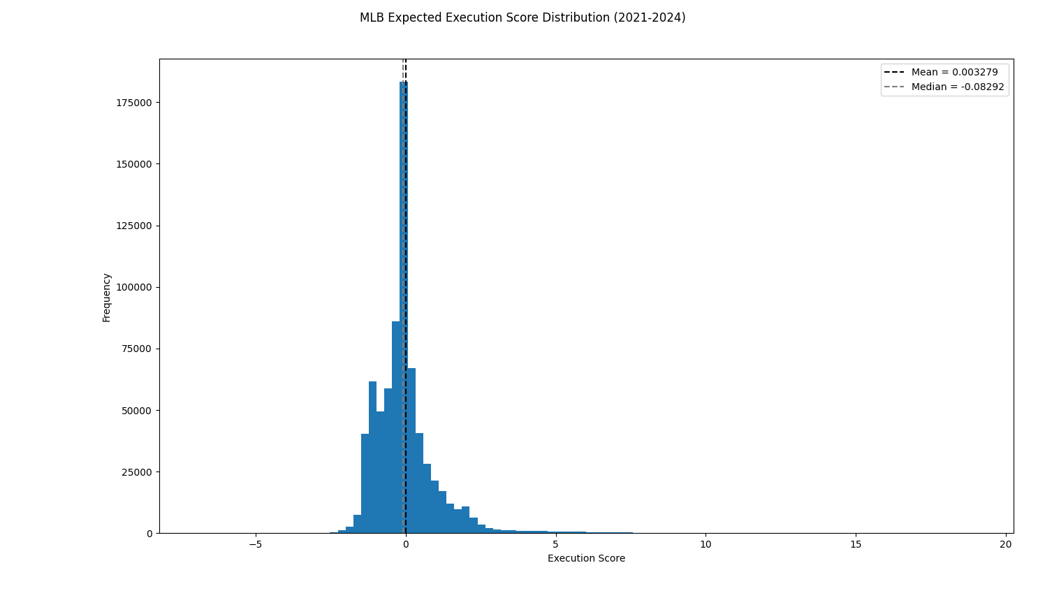
As expected, our distribution is still centered at 0. However, we notice that the distribution is smoother and more normally distributed than our raw Execution Score distribution.

We can also plot just the in-play at-bat scores, since those are the only values we modified:

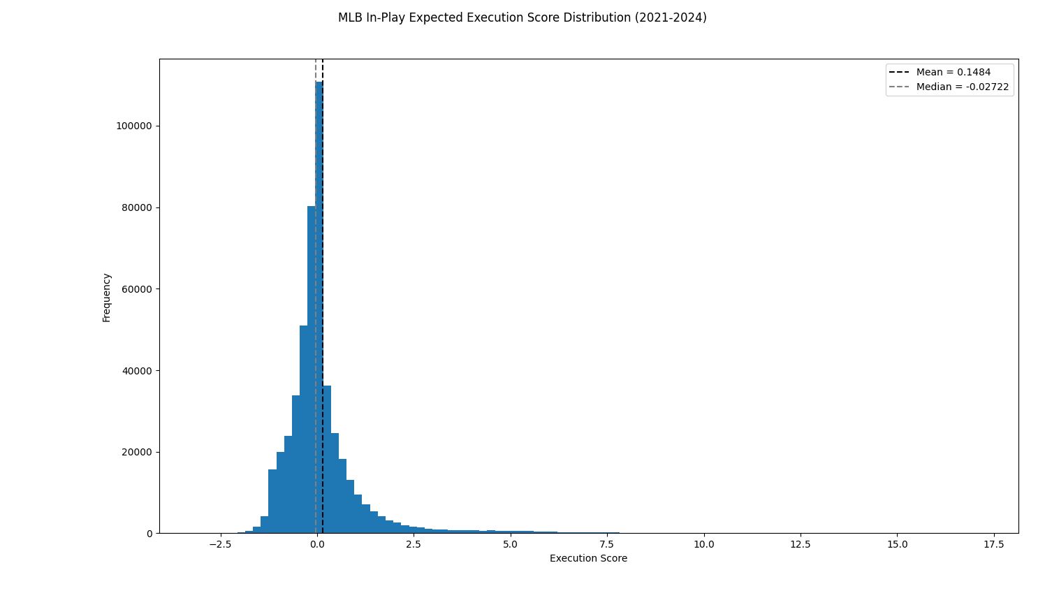
The mean of this distribution is positive, indicating that on-average, putting the ball in play has a positive net effect on Win Probability.

We can compare this distribution against the raw Execution Scores for in-play at-bats:

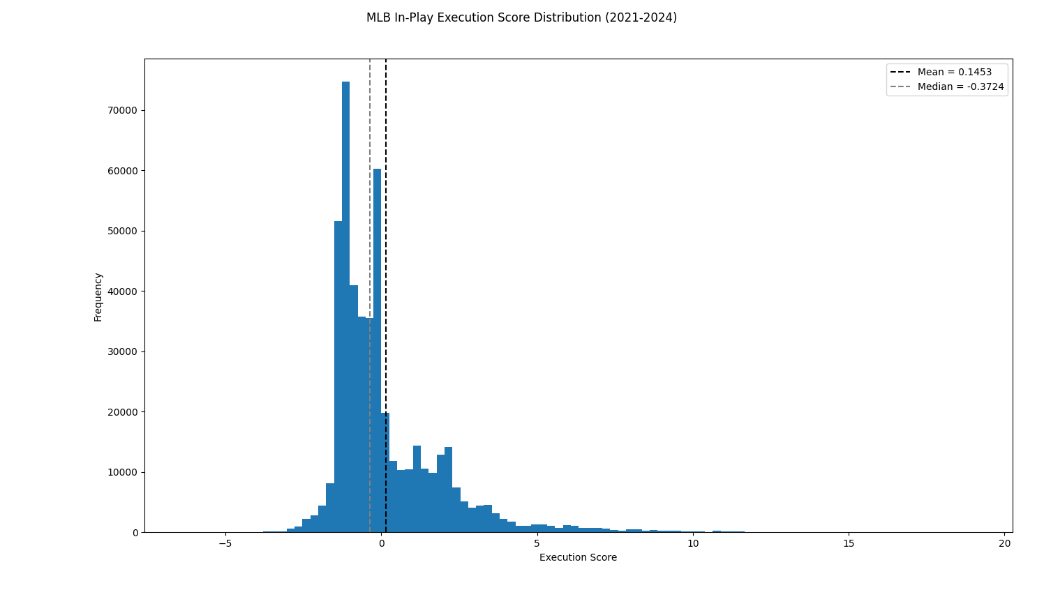
While the center is preserved, the distribution of Expected Execution Scores is much cleaner and nicer to work with.

As we did previously with raw scores, we can aggregate player Expected Execution Scores over a full season using the Log-Variance-Weighted method. Here is the leaderboard of expected scores for 2024 (minimum 300 at-bats):

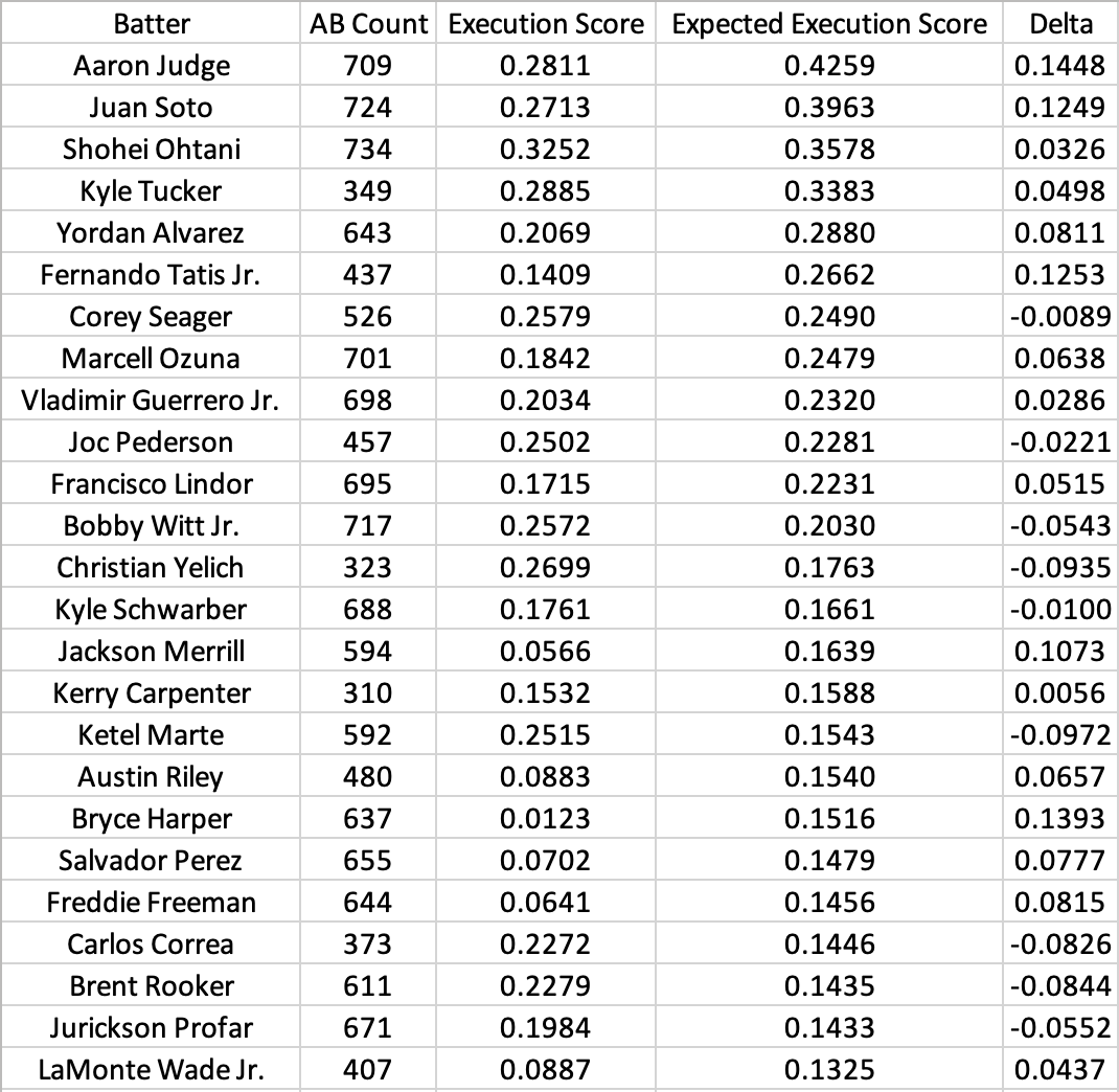
Using expected scores highlights just how incredible the offensive seasons Aaron Judge, Juan Soto, and Shohei Ohtani put together in 2024 really were. For those arguing for Bobby Witt as the AL MVP, we can see that Judge produced roughly double the net value of Witt per at-bat.

We can look at the delta between expected and raw scores as a measurement of general luck. Here are the “luckiest” batters:

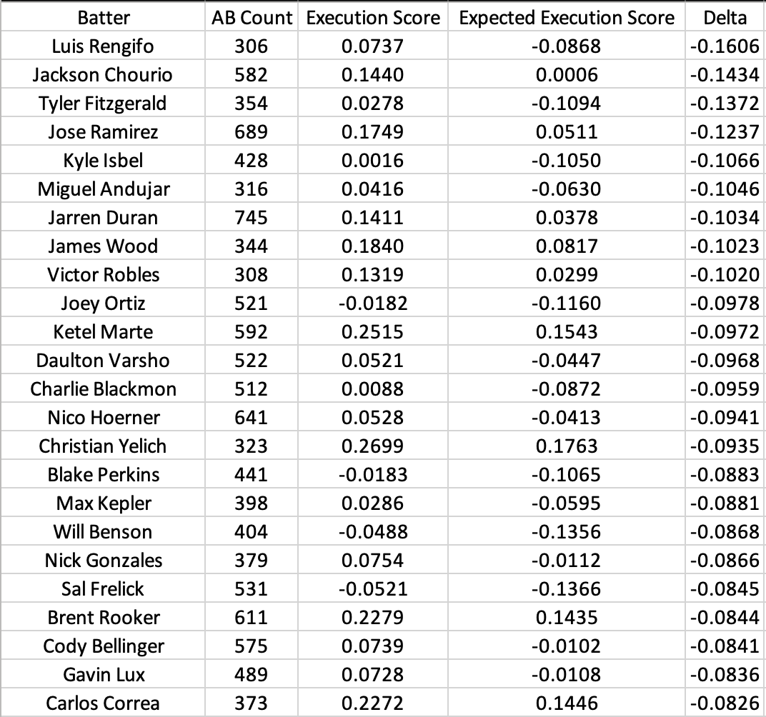
And here are the “unluckiest” batters:

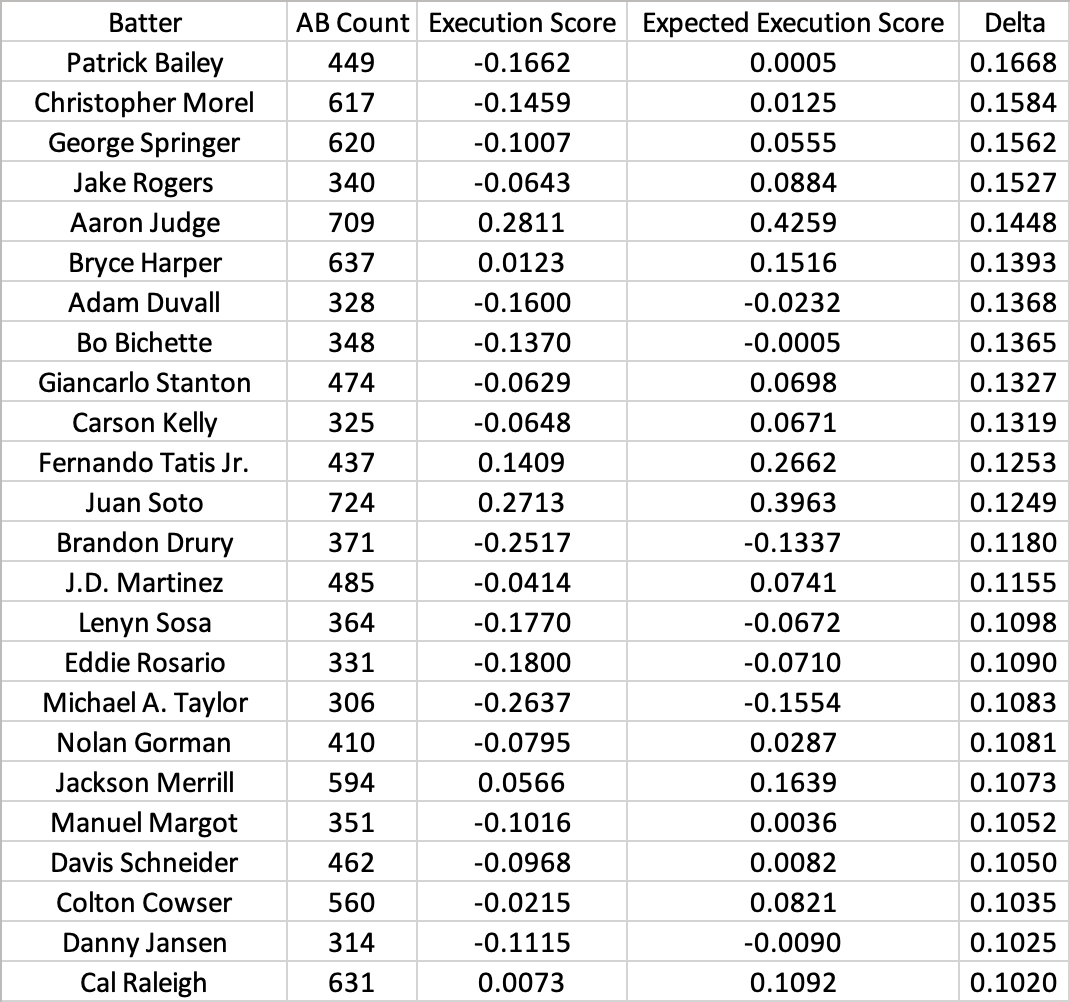
The “lucky” list appears to be skewed towards speedier contact hitters while the “unlucky” list is skewed towards power hitters. Notably, our feature set did not include any measurement of player speed, which would have increased the expected value of weak contact for faster players. We also used a relatively low polynomial degree (2), which had the effect of assigning more value to hard contact than hit placement. This demonstrates the impact of modeling decisions on expected scores.

However, we see that our final leaderboard is dominated by players who consistently hit for both power and average. While practitioners can tweak modeling assumptions to align with their baseball philosophies, Expected Execution Scores offer a robust framework to measure performance on both micro and macro levels.